Balaji | Code

Alpha Beta Matrix Multiplication!

Updated on: March 13, 2025

We have many methods to find matrix multiplication. Now, we will see the new one for square matrices.

We know what matrix multiplication is:

\begin{bmatrix} a & b & c \\ . & . & . \\ . & . & . \end{bmatrix} \times \begin{bmatrix} x & . & . \\ y & . & . \\ z & . & . \end{bmatrix} = \begin{bmatrix} ax+by+cz & . & . \\ . & . & . \\ . & . & . \end{bmatrix}

Here, if you see, we need to find a new sum every time, with no way to reuse previously computed values. We will try to reuse computations in our algorithm.

First, consider:

ax + by + cz = \alpha \cdot (a+b+c) \cdot (x+y+z) \quad \text{(Eq. 1)}

Where \( \alpha \) is a function that satisfies this equation.

We know that we can express any two-number product in the summation format:

n \cdot m = n + (m-1) \cdot n \quad \text{(Eq. 2)}

Apply Eq.2 in Eq.1:

Here, n = x, y & z and m = a,b & c

S_x + (a-1)x + (b-1)y + (c-1)z = \alpha \cdot S_a \cdot S_x

Where \( S_a \) is the sum of a, b, c and \( S_x \) is the sum of x, y, z.

Apply Eq.2 in Eq.1 for 'a' times:

aS_x + (b-a)y + (c-a)z = \alpha \cdot S_a \cdot S_x

Solving for \( \alpha \):

\alpha = \frac{a}{S_a} + \frac{(b-a)y + (c-a)z}{S_a S_x}

Let \( \beta = (b-a)y + (c-a)z \), then:

\alpha = \frac{a}{S_a} + \frac{\beta}{S_a S_x}

Now, we can reuse \( S_a \) and \( S_x \) in our calculations instead of performing full array multiplication every time.

This approach is really helpful when we use the same matrices repeatedly to calculate a new matrix with an existing matrix.

In the standard approach, we need to run O(n³) operations every time.

However, if we precompute constant values of our matrices, such as a/Sa, 1/Sa, and 1/Sx, we can reuse these values for consecutive matrix calculations.

With this method, precomputing values requires O(n²), and the main algorithm runs in O(n * n * (n - 1)).

For example, let's say we have matrices A, B, C, and D, and we need to perform multiple matrix multiplications. We assume that the same matrices will be used with different matrices, such as A*C, C*D, A*D, and C*B needed to calculate.

To run this in alpha beta algorithm, we calculate the constant values for each matrix, such as a/Sa, 1/Sa, and 1/Sx (if the matrix is on the right side of the multiplication). This allows us to reuse these values and perform matrix multiplication in O(n * n * (n - 1)).

For example, consider 5×5 matrices A, B, C, and D. We need to compute:

A*C, A*D, B*C, C*D, B*D, A*B

If we use the standard matrix multiplication approach:

A*C = 5³ = 125
A*D = 125
B*C = 125
C*D = 125
B*D = 125
A*B = 125

Total operations required: 750.

Using the optimized alpha-beta approach:

Precompute A, B, C, D: (5²) * 4 = 100
A*C = 5 * 5 * 4 = 100
A*D = 100
B*C = 100
C*D = 100
B*D = 100
A*B = 100

Total operations: 100 + (100 × 6) = 700.

Even for a small 5×5 matrix set, we saved 50 operations! As the number of matrices increases, the reduction in operations also increases.

Algorithm

1. Precompute for Left Matrix A:
a. Compute row-wise sums and store their inverses.
b. Compute first item fraction of each row.
c. Compute first item subtractions for all rows.

2. Precompute for Right Matrix B:
a. Compute column-wise sums and store their inverses.

3. Perform Alpha-Beta Matrix Multiplication:
a. For each row index in A:
i. Retrieve precomputed values.
b. For each column index in B:
i. Compute β using precomputed first-item subtractions.
ii. Compute α using β and precomputed values.
iii. Compute and store final matrix value in C.

C Implementation: View the full file here generated 🔗

Algorithm Performance Analysis

This reuse operation significantly helps my algorithm to beat the standard 3-loop algorithm.

I tested my code on one type of CPU architecture only. I need to check more about this.

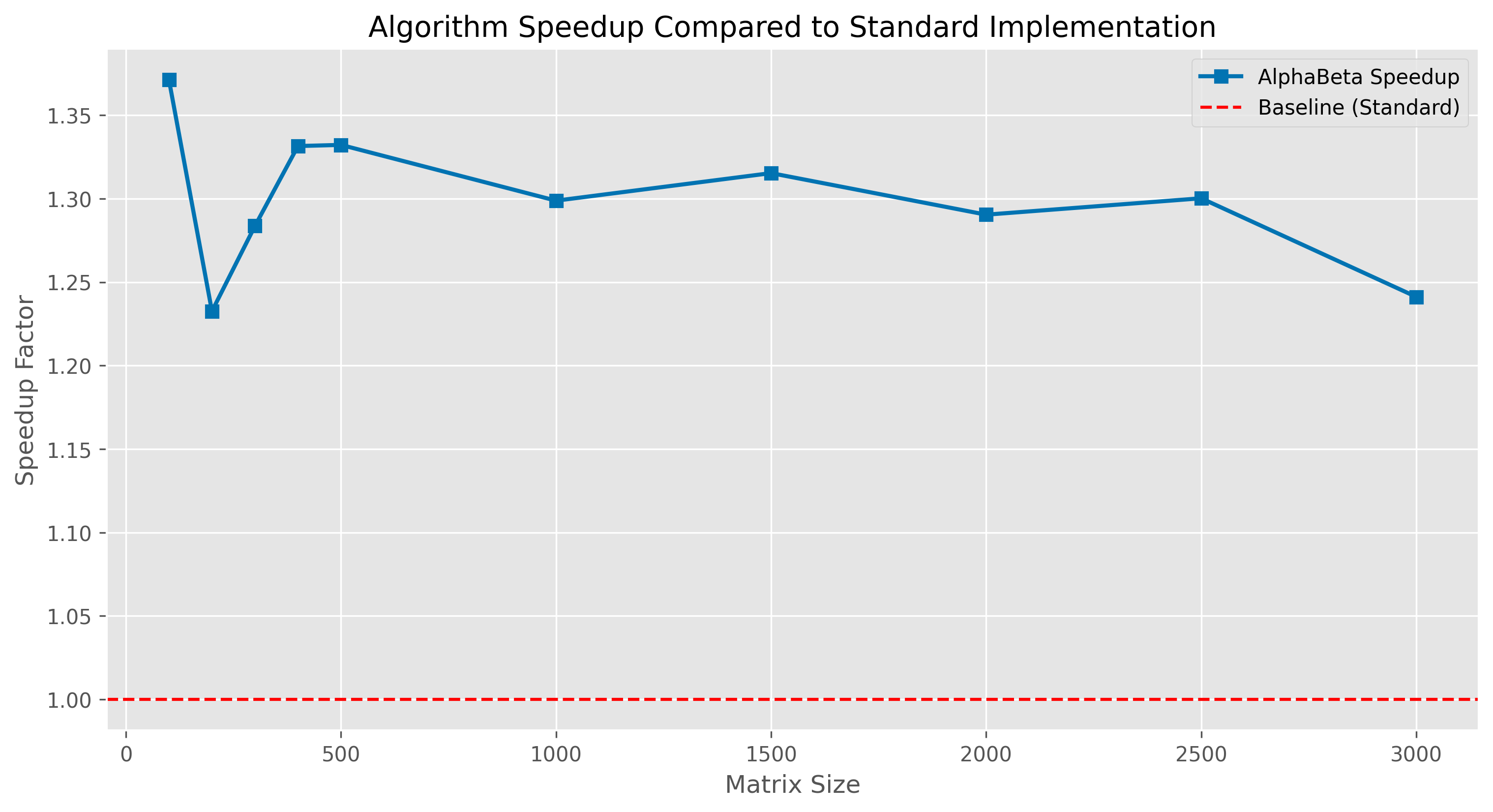
When I completed my testing on my machine, I noticed that my algorithm performed at an average speed of 1.28x compared to the standard 3-loop implementation in C (Thanks to ChatGPT & Claude AI for converting my Python code to C).

The next step is to test on different systems and environments. I also need to think about how I can format the beta value and separate the its multiplicative terms and memory consumption.

I am definitely using extra space, so I need to check how to reduce that.

When you simplify my equation, you will get ax + by + cz, the original equation. But instead of solving it directly, what I did was:

First, I looked for a way to reuse computed values.
For that, I created a dummy equation and started finding a balancer to make my dummy equation true.
This separation helps me reuse computed values and modify the existing standard algorithm.

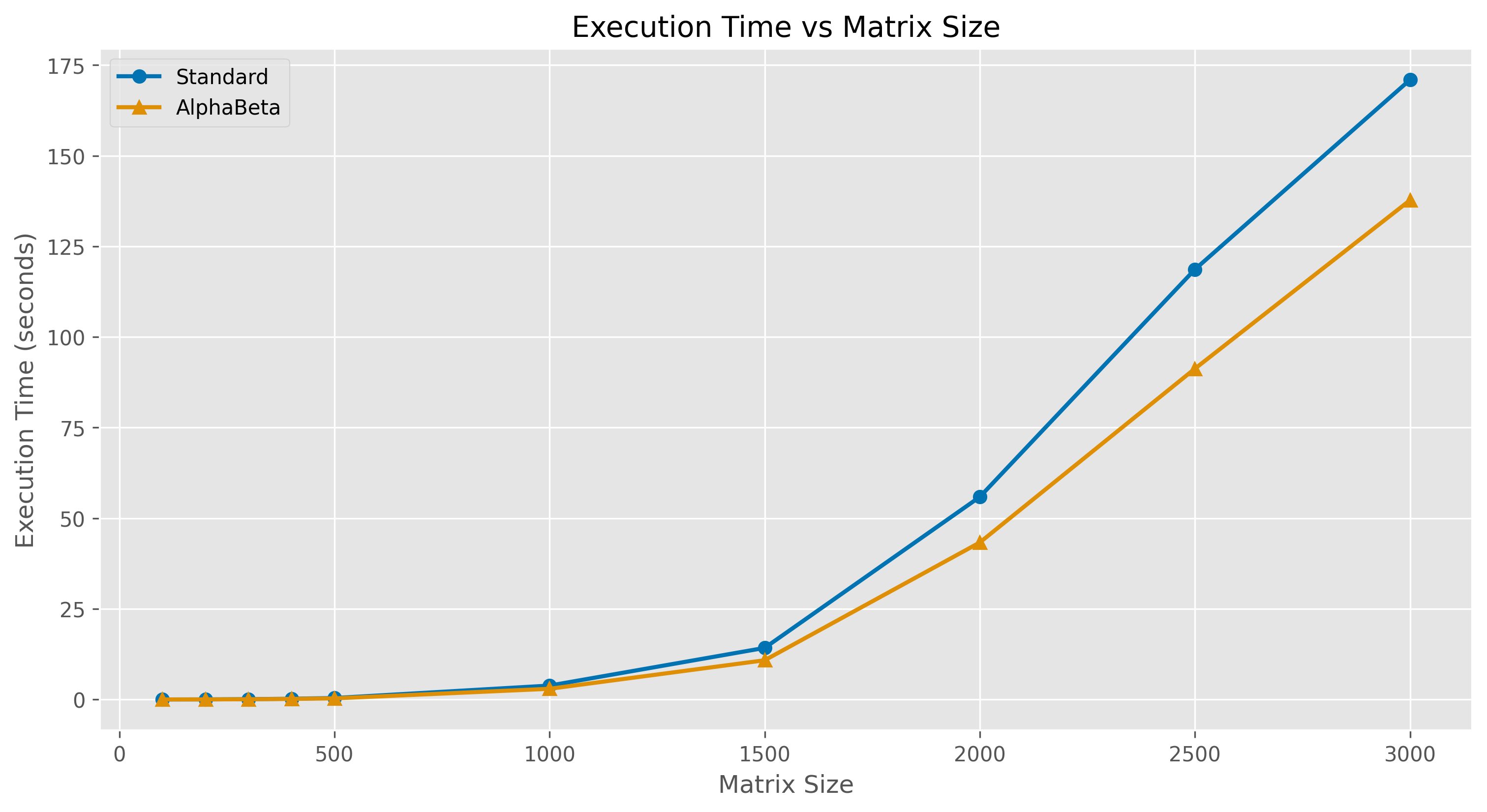
Dimension n*n	Standard Algorithm(sec)	AlphaBeta Algorithm(sec)	Speedup Factor
100	0.004429	0.003230	1.37x
200	0.022573	0.018314	1.23x
500	0.397208	0.298162	1.33x
1000	3.829336	2.948415	1.29x
1500	14.227654	10.817139	1.31x
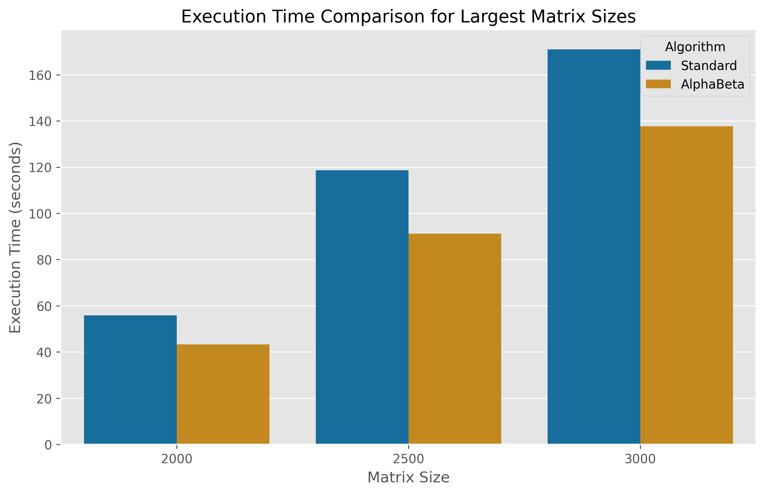
2000	55.889342	43.312036	1.29x
2500	118.649450	91.253632	1.30x
3000	170.963293	137.742198	1.24x

When you closely compare my algorithm and the standard one in C implementation, you will notice there is only one change:

In the innermost loop, I iterate only n-1 times. We calculate all the reusable values at the beginning of the calculations, and during multiplication, we use those values to achieve O(n * n * (n - 1)).

This algorithm has some limitations

This method applies only to two identical n × n matrices.
It will not give accurate results for decimal values.

I asked ChatGPT to find any real-time use cases similar to this, and found the following:

Machine Learning - Reusing weight matrices in inference (e.g., Transformers, neural networks).
Graph Processing - Faster adjacency matrix operations (e.g., PageRank, shortest paths).
Financial Modeling - Portfolio risk calculations with repeated data.
Physics Simulations - Real-time 3D transformations in robotics/games.
Traffic/Network Simulations - Optimizing routing using fixed structures.

For full detail explanation: Click here

Execution Time Comparison in C Implementation