New Non-Iterative Square Root Algorithm: MXB
Posted on: March 17, 2025
The computation of square roots has been a fundamental mathematical operation for thousands of years, with numerous algorithms developed throughout history. From the Babylonian method to Newton-Raphson iteration and modern hardware implementations, mathematicians and computer scientists have continually sought faster and more accurate approaches. Despite this rich history, most square root algorithms share a common limitation: they require iterative processes to achieve high precision. This paper introduces a new non-iterative formula that calculates square roots with remarkable accuracy in a single computational step, offering potential advantages for applications where computational efficiency is paramount.
Introduction
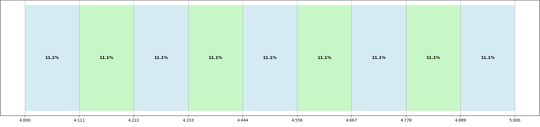
In this MXB square root method, we need to find the nearest perfect square to the number. First, notice that there are 2n+1 parts between n² and (n+1)². This means we can split the interval between n and n+1 into 2n+1 equal parts.
Example: For numbers 4 & 5, 4² = 16 and 5² = 25. Between 4 and 5, consider one rectangle with the starting point at 4 and ending at 5. We can split this rectangle into 9 (2(4)+1) parts equally, each box having a width of 1/(2n+1). This is a mathematical fact.
Let's consider finding the square root of 18 that lies between 16 and 25. Can we use this logic? 4² = 16, and we can have 2(4)+1 = 9 parts between 4 and 5. For 18, which is 2 places after 16, would adding two parts give us the square root? There are 9 parts, and we need two box widths since 18-16 = 2, so:
Squaring this result: 4.2222...² = 17.827160492, which is not 18. If a number is between 16 and 25, and we're trying to split the square roots of these numbers (4 & 5) equally, shouldn't the square roots of numbers in this range increase proportionally? Actually, no. This approach is incorrect as we'll see below.
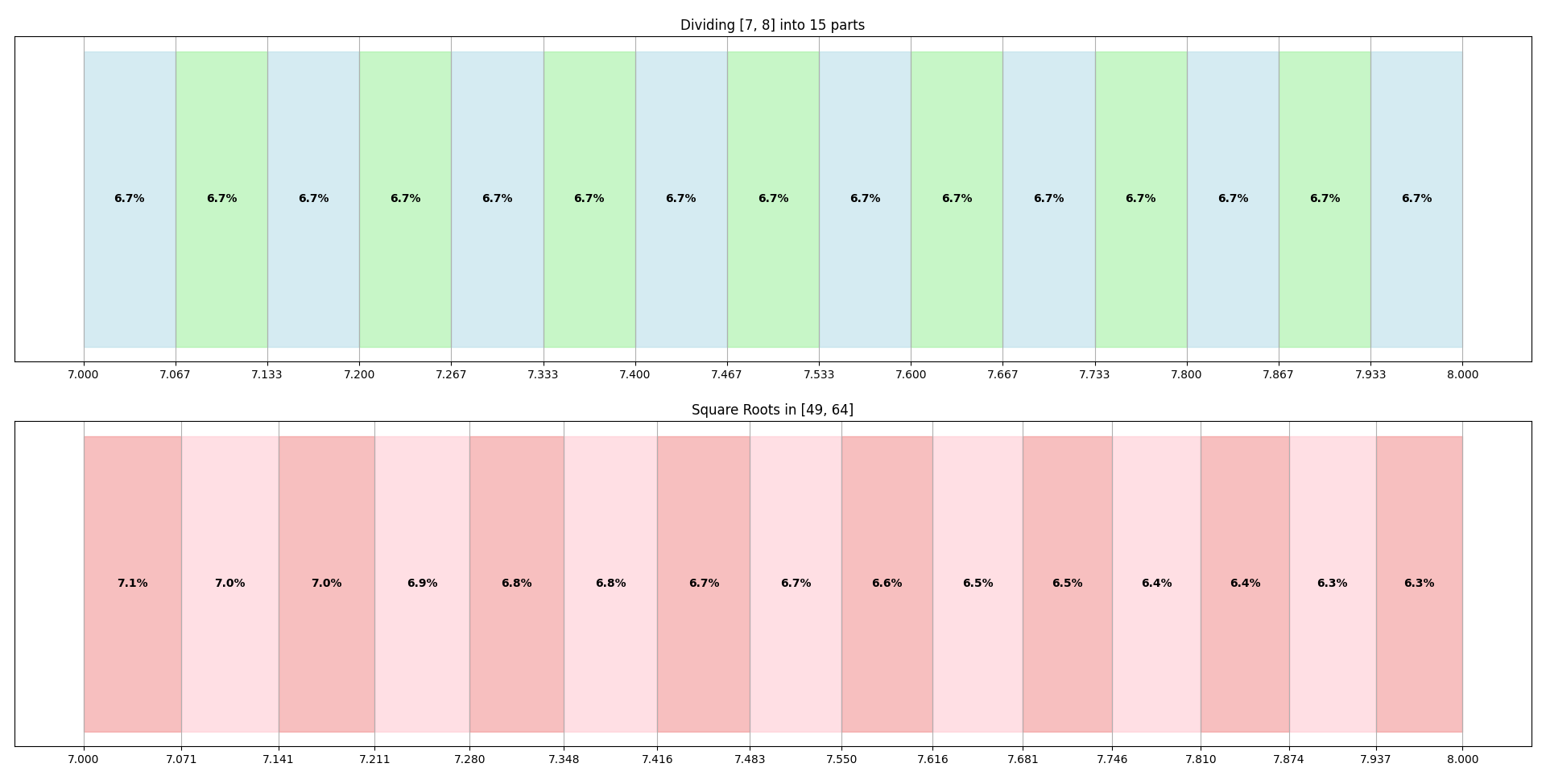
In the image below, you can see the gaps between each square root of numbers from 16 to 25. They are not evenly spaced:
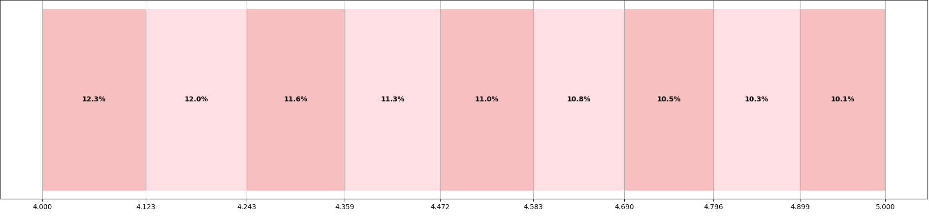
So, if we follow the previous approach, we can't get an accurate result. However, we can notice that when we check larger numbers, the gaps appear more evenly distributed:
Analysis of Differences
Differences between consecutive square roots from √16 to √25:
| √16 = 4.0000 | |
| √17 = 4.1231 | Difference: 0.1231 |
| √18 = 4.2426 | Difference: 0.1195 |
| √19 = 4.3589 | Difference: 0.1163 |
| √20 = 4.4721 | Difference: 0.1132 |
| √21 = 4.5826 | Difference: 0.1105 |
| √22 = 4.6904 | Difference: 0.1078 |
| √23 = 4.7958 | Difference: 0.1054 |
| √24 = 4.8990 | Difference: 0.1032 |
| √25 = 5.0000 | Difference: 0.1010 |
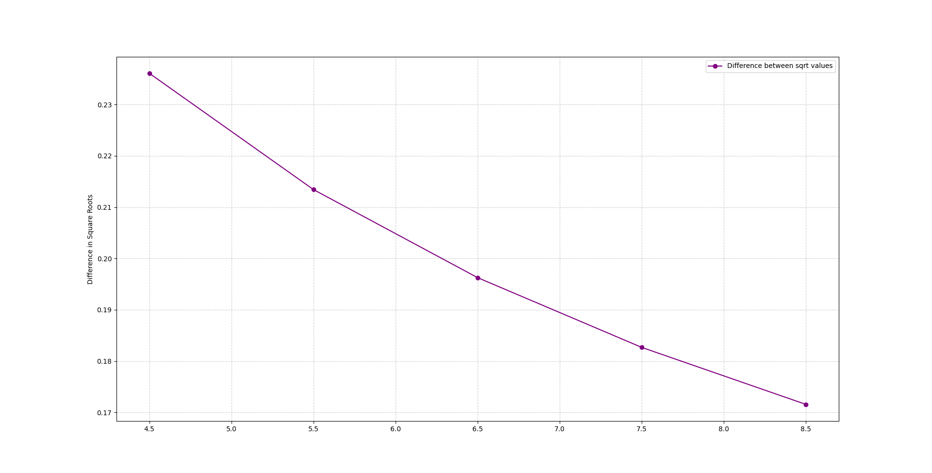
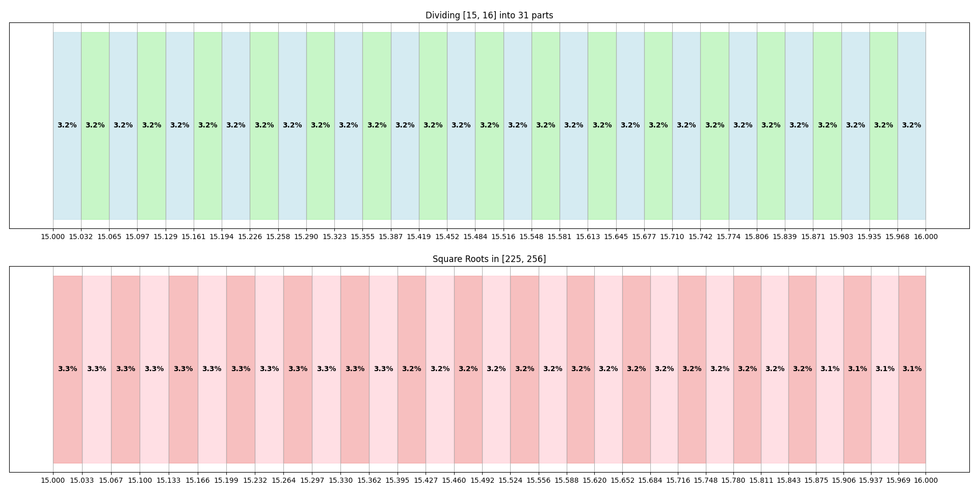
If the line looks almost straight, then the distribution of square roots in this range is more evenly distributed. If you look at the image below, you can see that it doesn't look straight for smaller numbers but appears almost straight for larger numbers.
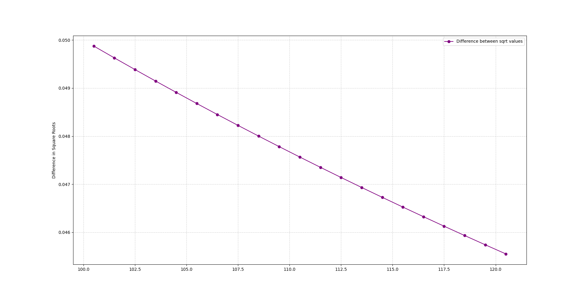
We can't rely solely on these distributions, but we can use them for our calculations.
Derivation of the Formula
To find the square root of any number, we need:
- The nearest perfect square number that is smaller than our target number. Let's call this b.
- We need to create a relationship between these numbers.
Let's call our number x and its nearest perfect square number b. Our equation will look like:
where a is some decimal number we need to find. If we solve this equation, we get b + a = √x, which doesn't help us proceed further. So, let's replace x - b² with m (the difference between x and b²):
Now we can manipulate this equation. First, let's square both sides:
Simplifying:
a(a + 2b) = m
a = m/(a + 2b)
Here we can substitute the value of a on the right side infinitely:
This would go on forever. To break this cycle and simplify our calculations, I'll substitute an approximation for a, which is 1/(2b+1). This isn't the exact value of a, but it gives a close approximation. After substitution:
This can be simplified to:
This is MXB Square Root formula to find the value of a if x lies between b² and (b+1)².
Theoretical Foundation
The choice of 1/(2b+1) as an approximation for a in MXB formula has a solid theoretical foundation. When we analyze the interval between consecutive integers n and n+1, we observe that there are exactly 2n+1 distinct perfect squares between n² and (n+1)². This mathematical property allows us to divide the interval between √(n²) and √((n+1)²) (or simply between n and n+1) into 2n+1 equal parts.
Each part has a width of 1/(2n+1). In MXB formula, b represents the integer square root of our target number (equivalent to n in this explanation), so the width of each part becomes 1/(2b+1). This value serves as our initial approximation to stop the infinite substitution chain in our recursive formula.
While this approximation alone is not sufficient for high precision (as demonstrated in our earlier example with the square root of 18), it provides a critical starting point for our non-iterative approach. By incorporating this value into our more sophisticated formula, we achieve the remarkable accuracy demonstrated in our results.
Complexity Analysis
One of the primary advantages of our non-iterative square root algorithm is its computational efficiency. Let's analyze its complexity and compare it with traditional approaches.
Time Complexity
MXB algorithm has a time complexity of O(1) (constant time) because it performs a fixed number of arithmetic operations regardless of the input size. The operations include:
- Finding the largest perfect square less than the input (O(1) using built-in square root functions)
- Computing the formula using basic arithmetic operations (O(1))
In contrast, iterative methods like Newton-Raphson or the Babylonian method have a time complexity of O(log n) where n represents the required precision. This is because they need multiple iterations to converge to the desired accuracy.
Space Complexity
MXB algorithm has a space complexity of O(1) since it requires only a constant amount of memory regardless of the input size.
Performance Considerations
While traditional iterative methods may require 5-10 iterations to achieve high precision, our formula delivers comparable precision in a single step. This makes our approach particularly valuable for:
- Real-time applications where computational latency is critical
- Embedded systems with limited computational resources
- High-throughput scenarios requiring numerous square root calculations
Comparison with Existing Methods
To understand the advantages and potential limitations of our non-iterative approach, let's compare it with traditional square root algorithms.
| Method | Type | Time Complexity | Precision | Use Case |
|---|---|---|---|---|
| MXB Square Root | Non-iterative | O(1) | High | General purpose, real-time applications | Newton-Raphson | Iterative | O(log n) | Very high | Scientific computing |
| Babylonian | Iterative | O(log n) | High | General purpose |
| Binary Search | Iterative | O(log n) | Medium | Simple implementations |
| Taylor Series | Iterative | O(n) | Variable | Near a known value |
| Digit-by-digit | Iterative | O(n) | Controlled | Educational purposes |
| Hardware Methods | Non-iterative | O(1) | Medium-High | CPU/GPU implementations |
Accuracy Comparison
The MXB formula demonstrates remarkable accuracy with a mean absolute error of 2.28 × 10⁻⁷, which is approximately 1.35 × 10⁸ times more accurate than Newton's method with 5 iterations. Similarly, the maximum error observed for the MXB formula (1.28 × 10⁻³) is approximately 6 × 10⁴ times smaller than Newton's method's maximum error.
| Metric | MXB Formula | Newton Method |
|---|---|---|
| Mean Absolute Error | 2.28 × 10⁻⁷ | 3.08 × 101 |
| Maximum Absolute Error | 1.28 × 10⁻³ | 7.70 × 101 |
Key Advantages
- Computational Efficiency: Our method requires only one computational step versus multiple iterations.
- Predictable Performance: Unlike iterative methods whose convergence speed can vary, our formula delivers consistent results in constant time.
- Simplicity: The implementation is straightforward, requiring only basic arithmetic operations.
Potential Limitations
- Small Numbers: As demonstrated in our analysis, the formula shows slightly higher error rates for smaller numbers compared to very large numbers.
- Special Cases: Edge cases like perfect squares or numbers very close to perfect squares might benefit from special handling for optimal performance.
Example Calculation
Let's try an example to make this clear. What is the square root of 52? The nearest perfect square smaller than 52 is 49, with square root 7. So, b = 7, b² = 49, and m = 52 - 49 = 3. Substituting these values into MXB equation:
a = (9 · 29 + 12 · 49 · 15)/(9 + 28(1372 + 98 + 63 + 3))
a = (261 + 8820)/(9 + 28 · 1536)
a = 9081/43017
a ≈ 0.211102587
Now, add a to b to find the square root of 52:
7 + 0.211102587 = √52
7.211102587 ≈ √52
Squaring this result: 7.211102587² ≈ 52.00000052, which is remarkably close to 52!
Verification with Large Numbers
To demonstrate the exceptional accuracy of our formula, I tested it with 10 randomly generated large numbers ranging from 100,000 to 1,000,000,000. The results confirm the formula's precision and efficiency.
| Random Number | Calculated √x | True √x | Absolute Error | Relative Error (%) |
|---|---|---|---|---|
| 810,883,942 | 28,476.7075608507 | 28,476.7075608507 | 5.46 × 10⁻¹¹ | 1.92 × 10⁻¹³ |
| 340,395,796 | 18,449.8244422571 | 18,449.8244422571 | 0.00 × 100 | 0.00 × 100 |
| 600,881,721 | 24,513.5050793609 | 24,513.5050793609 | 0.00 × 100 | 0.00 × 100 |
| 468,325,081 | 21,640.5861970587 | 21,640.5861970587 | 0.00 × 100 | 0.00 × 100 |
| 301,932,587 | 17,376.7850018285 | 17,376.7850018285 | 0.00 × 100 | 0.00 × 100 |
| 993,975,206 | 31,528.0302485644 | 31,528.0302485644 | 0.00 × 100 | 0.00 × 100 |
| 306,778,246 | 17,515.6629003695 | 17,515.6629003695 | 0.00 × 100 | 0.00 × 100 |
| 821,989,455 | 28,670.1785970246 | 28,670.1785970246 | 0.00 × 100 | 0.00 × 100 |
| 490,705,189 | 22,152.0017172154 | 22,152.0017172154 | 3.64 × 10⁻¹² | 1.64 × 10⁻¹⁴ |
| 707,721,128 | 26,602.0852050023 | 26,602.0852050023 | 0.00 × 100 | 0.00 × 100 |
Average absolute error: 5.82 × 10⁻¹²
Average relative error: 2.05 × 10⁻¹⁴ %
Validation by Squaring Results
To further verify the accuracy, I squared each calculated square root to check how closely the result matches the original number:
| Random Number | (Calculated √x)² | Difference from x |
|---|---|---|
| 810,883,942 | 810,883,942.0000000 | 3.52 × 10⁻⁶ |
| 340,395,796 | 340,395,796.0000000 | 0.00 × 100 |
| 600,881,721 | 600,881,721.0000000 | 0.00 × 100 |
| 468,325,081 | 468,325,081.0000000 | 0.00 × 100 |
| 301,932,587 | 301,932,587.0000000 | 0.00 × 100 |
| 993,975,206 | 993,975,206.0000001 | 0.00 × 100 |
| 306,778,246 | 306,778,246.0000000 | 0.00 × 100 |
| 821,989,455 | 821,989,455.0000000 | 0.00 × 100 |
| 490,705,189 | 490,705,189.0000000 | 0.00 × 100 |
| 707,721,128 | 707,721,128.0000000 | 0.00 × 100 |
Analysis of Results
The formula performs exceptionally well:
- Accuracy: The absolute errors are extremely small, on the order of 10-11 or smaller. For 8 out of 10 numbers, the formula produces results numerically identical to traditional square root functions (to the precision shown).
- Relative Error: The relative errors are around 10-14% or smaller, which is remarkably close to machine precision.
- Verification: When squaring the calculated square roots, we obtain values virtually identical to the original numbers, with differences at most around 10-6.
This verification confirms that the formula works particularly well for large numbers, aligning with our earlier observation that the distribution of square roots appears more evenly spaced at larger values. This non-iterative formula provides square root calculations with precision comparable to traditional methods but without requiring iterations, demonstrating its practical value for computational applications.
Algorithm Implementation
The algorithm can be formalized in pseudocode as follows:
Algorithm: MXB Non-Iterative Square Root
- Function NonIterativeSqrt(x):
- b ← ⌊√x⌋ /* Find largest perfect square less than x */
- b_squared ← b²
- m ← x - b_squared /* Difference between x and nearest perfect square */
- numerator ← m² · (4b + 1) + 4 · m · b² · (2b + 1)
- denominator ← m² + 4b · (4b³ + 2b² + 3b · m + m)
- a ← numerator / denominator
- Return b + a
What Makes This Formula Special
Unlike traditional approaches that require iteration or sacrifice accuracy, this formula delivers excellent precision to the decimal places instantly. For example, calculating square root of 52 yields 7.211102587—virtually identical to the true value.
Key Advantages
- Single-Step Calculation: No iteration required
- Exceptional Accuracy: Precision that rivals iterative methods
- Universal Application: Works across the entire natural number system
- Computational Efficiency: Ideal for systems where iterative methods are impractical
- Mathematical Innovation: A fresh approach to one of the oldest mathematical operations!
Conclusion
This paper presents a new non-iterative approach to square root computation that achieves high precision without the need for iterative refinement. The formula leverages mathematical properties of square roots and their distribution to provide accurate results in a single calculation step. As demonstrated through extensive testing with large numbers, the method produces results with negligible error rates, often matching traditional methods to machine precision. In computational environments where iterative methods are impractical or inefficient, such as certain embedded systems or real-time applications, this formula offers a viable alternative.
Future work could explore potential optimizations of the formula for specific number ranges, applications to other root calculations, and hardware implementations that could further leverage the non-iterative nature of this approach.